Essential Functions
Reading/Writing Data
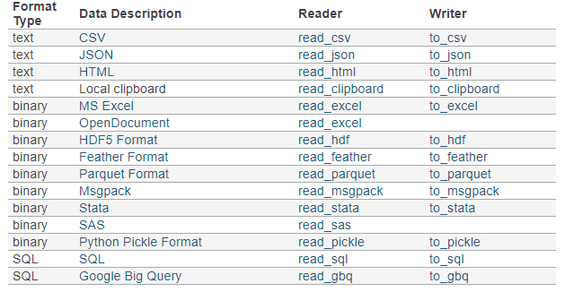
Pandas can handle virtually any data file format. Below is a table containing supported data formats and their reader & writer functions.
Import Parameters
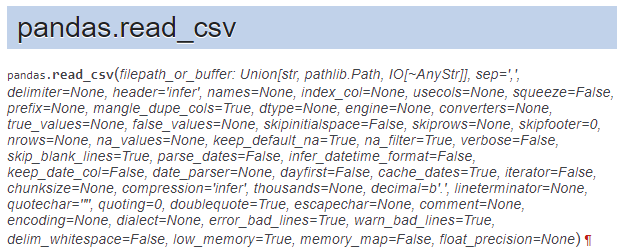
It has more than 50 parameters!? Here are some important parameters you might need to pay attention to.
- filepath_or_buffer: Any valid string path is acceptable. The string could be a URL. for example: Windows: "D:/data/xx.csv" OS: "usr/you/document/xxx.csv"
Tip: for Mac users, if you do not know the path of a file, you could simply drag the target file into a terminal. The prompt tells you the path of that file. - sep: Separator/delimiter to use to parse the file. Defaults to ','. If your data is TSV (tab-separated values) file, pass '\t' to this parameter.
- header: the row number to use as column names. Defaults to 'infer'. If your data has no columns present in the file, set this parameter to None and also pass a list of names to the name parameter.
- names: used when your data has no columns.
- usecols: return a subset of the columns. Instead of reading the whole dataset, this parameter tells pandas to read the columns of your interest. It is particularly useful when you are dealing with a massive dataset.
- encoding: defaults to 'utf-8'. check here to get a list of all supported encodings.
import pandas as pd
import numpy as np
data = pd.read_csv(filepath_or_buffer='data/titanic.csv')#change the file path accordingly or use the URL address
data.head()
Exploring Data
The first thing to do after your data is loaded into Notebook, is to get to know the basic information (e.g., the dimension, size, shape, data types of all the columns) of your data and what your data looks like roughly. All the basic information can be retrieved from DataFrame object's attributes.
Hint: What are attributes of an object? Attributes are the info/properties pre-calculated when you instantiate an object.
Getting the basic info of the data through attributes
- shape: return a tuple representing the dimensionality of the Dataframe
- ndim: return an integer representing the number of dimensions
- dtypes: return a Series including the data type of each column of the DataFrame.
- index: Return the index (also known as row labels) of the Dataframe
- columns: return a list of column names
#Example: Here I am using some Numpy functions to manually create a 2-d array and then transform it to a DataFrame instance.
#You could skip over this step and simply use the Titanic data.
data = pd.DataFrame(np.random.randint(0,10, (4,3)),
                    columns= ['col1', 'col2','col3'],
                   index=['row1','row2','row3','row4'])
data.shape
data.ndim
data.dtypes
data.index
data.columns
Viewing the data
- head(n): return the first n rows. It is a quick solution to get a good sense of data and also to test if your data is loaded as you expect. The parameter n defaults to 5.
- tail(n): return the last n rows. The parameter n defaults to 5.
- describe(percentile = None, include=None, exclude=None): Generate descriptive statistics of the included columns that summarize the central tendency, dispersion, shape, ignoring NaN values. By default, this summarization only applies to numeric columns.
- mean(), sum(),min(), max(), idxmin(), idxmax(): get the mean, sum, minimum, maximum, the index of the minimum value, the index of maximum value of all columns
#Example
data = pd.DataFrame(np.random.randint(0,10, (4,3)),
                    columns= ['col1', 'col2','col3'],
                   index=['row1','row2','row3','row4'])
data.head(2)
data.tail(1)
data.describe()
data.mean()
data.sum()
data.max()
data.idxmax()
Indexing: Selecting, Slicing and Modifying Data
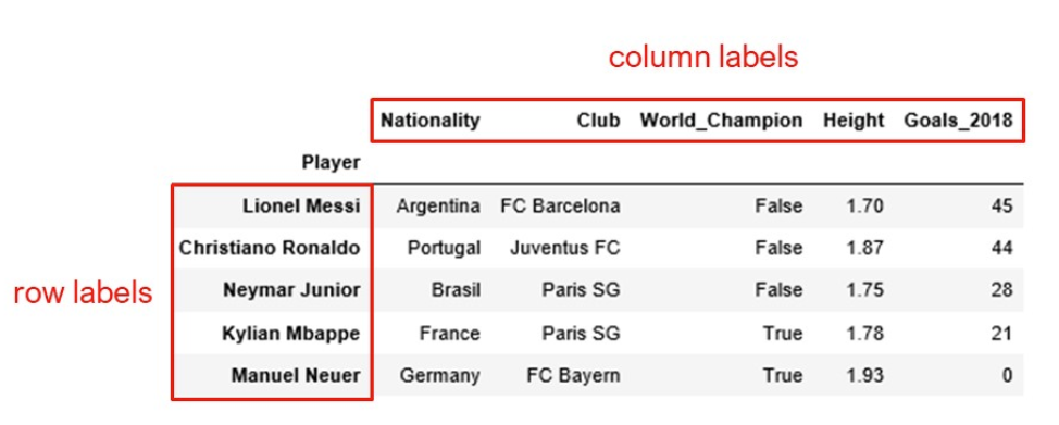
Pandas has two indexing systems. One is the position-based indexing and the other is the label-based indexing. While dealing with Series or DataFrame objects, you can use either positions (like what you do with Python on indexing a list) or label for selecting, slicing and modifying values.
Position-based Indexing System
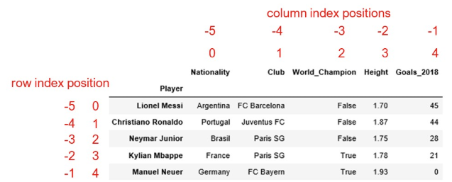
Label-based indexing System
Two methods for indexing
- .iloc[]: position-based method for indexing. Allowed inputs are:
- An integer, e.g. 5.
- A list or array of integers, e.g. [4, 3, 0].
- A slice object with ints, e.g. 1:7.
- A boolean array.
- A callable function with one argument (the calling Series or DataFrame) and that returns valid output for indexing (one of the above). This is useful in method chains, when you don’t have a reference to the calling object, but would like to base your selection on some value.
- .loc[]: label-based method for indexing. Allowed inputs are:
- A single label, e.g. 5 or 'a', (note that 5 is interpreted as a label of the index).
- A list or array of labels, e.g. ['a', 'b', 'c'].
- A slice object with labels, e.g. 'a':'f'. Warning: Contrary to usual python slices, For the slice in Pandas, both the start and the stop slice bounds are included.
- A boolean array of the same length as the axis being sliced, e.g. [True, False, True].
- A callable function with one argument (the calling Series or DataFrame) and that returns valid output for indexing (one of the above)
What is a boolean array? (Aka Boolean Mask array)
A boolean array is an array filled with True or False values. It is primarily used as a mask indicating whether the corresponding entries is selected or not.
#Example
data = pd.DataFrame(np.random.random((4,5)))
data
mask_row = [True, False, False, False]
data.iloc[mask_row,:] # data.loc[mask_row,:] also works
mask_column = [True, True, False,False, False]
data.iloc[:, mask_column] # data.loc[:, mask_column] also works
data.loc[:, mask_column]
##A step further: We want to select rows whose first column>0.4
data.loc[data.iloc[:,0]>0.4]
#decompose the compound statement above.
# The same effect can be accompolished by the following code
mask = data.iloc[:,0]>0.4
data.loc[mask]
Pre-processing Data
Before you start to analyze your data, you might realize that you have to spend a large amount of time cleaning up data. The possible cleansing operations can be:
1. dropping irrelevant columns/rows,
2. adding new columns/rows,
3. fixing data missings,  dropping columns/rows in which too many missing entries are present
4. transforming certain columns E.g., add 100 to column x.
Column-related Operations:
- .drop(columns=, inplace=False): Drop columns by names, pass a list of names to the parameter columns. If inplace is True, the changes is operated on the original data, otherwise, a copy will be returned.
- .dropna(axis='columns', how='any', thresh=None, subset=None, inplace=False) Drop columns by missings. Threshold: the minimum number of non-Nan values. subset: labels along other axis to consider.
- .insert(loc, column, value): Add a new column. loc: the insertion index. Must be between 0 and len(columns)
- .rename(columns={oldname: newname, }, inplace=False) Rename columns:
- data.column-name.apply(func) : apply a transformation function to a certain column.
#Example
data = pd.DataFrame(np.random.random((4,5)),
                    columns=['col_'+str(x) for x in range(5)],
                   index=['row_'+str(x) for x in range(4)])
data
#drop col_0 column
data.drop(columns='col_0')
data # why col_0 is still in there?
#before we use dropna method, let's add some nan values to col_1 by using loc method
data.loc['row_0','col_1'] = np.nan
data
data.dropna(axis='columns', how='any')
data #Rule 1: Most operations generate a copy.
data.dropna(axis='columns', how='any', inplace=True) #Rule 2: if inplace parameter is present in a function, it allows you to make a inplace change.
#insert a new column
data.insert(value=np.random.random(4), column='col_new',loc=0 )
data
#rename col_new to col_new2
data.rename(columns={'col_new':'col_new2'},inplace=True)
data
## Apply a function to each column to do transfromations.
#Tip: you can use a attribute-style to reference a column. E.g., data.A
#e.g., add [1,2,3,4] to col_new2
data.col_new2.apply(lambda x: x+10)
# wait!!!! what is that? How come I get a Series object? I was expecting to get a updated dataframe.
# Remember Rule 1? Every operation generates a copy.
data.col_new2 = data.col_new2.apply(lambda x: x+10) #rewrite the column col_new2
data
Row-related Operations:
- .drop(index=, inplace=False): Drop rows by labels, pass a list of names to the parameter index. If inplace is True, the changes is operated on the original data, otherwise, a modified copy is returned.
- .dropna(axis='index', how='any', thresh=None, subset=None, inplace=False) Drop rows by missings. Threshold: the number of non-Nan values. subset: labels along other axis to consider.
- .append(other, ignore_index=False): Add another DataFrame to the end of the current DF. if ignore_index=True, the index of the output is reset.
- .rename(index={oldname: newname, }, inplace=False) Rename row labels:
- .apply(func, axis=1, ) : apply a transformation function to each row. for instance, get the sum of each row.
data = pd.DataFrame(np.random.rand(4,5),
                    columns=['col_'+str(x) for x in range(5)],
                   index=['row_'+str(x) for x in range(4)])
data
#drop the first row
data.drop(index='row_0')
data
#add some missing values to the row_2
data.loc['row_2',['col_0','col_1','col_2']]=np.nan
data
#drop the rows in which the the number of Non-nan is less than the threshold
data.dropna(axis=0, thresh=3)
data.rename(index={'row_0':'row_new'})
#try append function
data2 = pd.DataFrame(np.random.rand(4,5),
                    columns=['col_'+str(x) for x in range(5)],
                   index=['row_'+str(x) for x in range(4)])
data2
data.append(data2, ignore_index=False)
data.append(data2, ignore_index=True)
#apply a transformation to each values of each row
data.apply(func=lambda x: x+[0, 1, 2, 3, 4], axis=1)
Element-related Operations:
- .applymap(func): apply a function to each element of the dataframe
#get the length of each element
data = pd.DataFrame(np.random.randint(0,100, (4,3)),
                    columns=['col_'+str(x) for x in range(3)],
                   index=['row_'+str(x) for x in range(4)])
data
data.applymap(lambda x: x*2)
Missing value
- .isull(): element-wise operation. Detect if a value is np.nan. Tip: np.nan is a data type notation to representing nullnuess in Numpy.
- .notnull(): element-wise operation. The opposite of isnull()
- .fillna(value=None, method=None, axis=None,inplace=False) Fill Nan values using specified value(s) or method
Count how many missings are present in each column
data = pd.DataFrame(np.random.randint(0,100, (4,3)),
                    columns= ['col_'+str(x) for x in range(3)],
                   index = ['row_'+str(x) for x in range(4)])
data.iloc[[2,3],[0,1]] = np.nan
data
data.isnull()
data.notnull()
#Count how many missings are present in each column
data.isnull().sum()
#Count the number of non-missings in each column
data.notnull().sum()
fill missings with 0s
data = pd.DataFrame(np.random.randint(0,100, (4,3)),
                    columns=['col_'+str(x) for x in range(3)],
                   index=['row_'+str(x) for x in range(4)])
#add some missings
data.iloc[[0,1],[0,1]] = np.nan
data
data.fillna(value=0)
fill missings with column means
data.fillna(value=data.mean(), axis=0)
Fill missing with backward-fill method
data.fillna(axis=0, method='backfill')
Merging/Joining Data
- .merge(right, how='inner', on=None, left_on=None, right_on=None, left_index=False, right_index=False, ): merge two dataframe objects on the specified column/index.
.join(other, on=None,lsuffix='', rsuffix=''): Similar to the merge function, with the exception that join method only uses the index of other dataframe objects.
Merge Vs Join:
- Merge gives you more customization power than join. You could tell this from the number of parameters. Merge method has more parameters than join function.
- Join only uses the index of the other dataframe objects, however merge can use either index or a column.
- The biggest advantage of using join is that you could join as many dataframes as possible, only when you want to align data by index.
data1 = pd.DataFrame(np.random.randint(0,10, (4,3)),
                     columns= ['col_'+str(x) for x in range(3)],
                     index=['row_'+str(x) for x in range(4)])
data2 = pd.DataFrame(np.random.randint(0,10, (4,3)),
                     columns= ['col_'+str(x) for x in range(3)],
                     index=['row_'+str(x) for x in range(4)])
data1
data2
"Join" two dataframes using index
data1.join(data2, rsuffix='_r')
"Merge" two dataframes using index
#merge two dfs on the index, same as the join
data1.merge(data2, left_index=True, right_index=True)
Merge two dataframes on a common column
#merge two dfs on a specified common column,
data1.merge(data2, on='col_2')
Iteration of DataFrame
- Iterate over rows:
- iterrows(): return a pair(index, Series)
- itertuples(): return a named tuple object: Pandas(Index=0, col_1=2, ...) (Recommended as this method preserves the data types of values)
- Iterate over columns:
- iteritems(): return a pair (column name, Series) paris
data = pd.DataFrame(np.random.randint(0,10, (4,3)),
                     columns= ['col_'+str(x) for x in range(3)],
                     index=['row_'+str(x) for x in range(4)])
data
Iteration over rows
##Example: iterate over rows
for row in data.itertuples():
    print(row.Index, row.col_2)
#Example iterate over rows using iterrows
for i, row in data.iterrows():
    print(row.col_2)
Iteration over columns
#example iterate over columns
for col in data.iteritems():
    print(col) #col is a series object
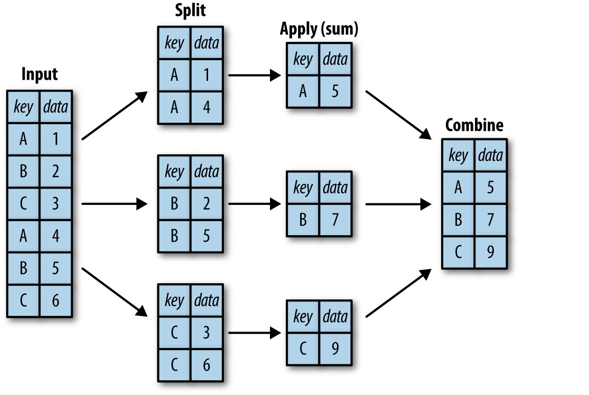
GroupBy Operations
.groupby(by=None). The parameter by is used to dtermine how to make groups. The canonical example is by = a column name.
A groupby operation is a combination of splitting the object into groups, applying a function to each group, and combining the results.
- The splitting step breaks up the dataframe into groups depending on the values of the specified key.
- The applying step does some computing operations (e.g., transformation, aggregation(sum, std),) within each group.
- The combining step merges the results of all the groups into an output dataframe.
#Example
data = pd.DataFrame({'name':['p1','p2','p3','p4','p5'],
    'state':['TX',"RI","TX","CA","MA"],
                     'income(K)':np.random.randint(20,70,5),
                    'height': [4, 5, 6.2, 5.2, 5.1]})
data
#get the mean income of each state
data.groupby('state').mean() # Question: where is name? mean operation is not compatible with a string column.
data.groupby('state').sum()
#what if we want to get the max of the column income and min of column height
data.groupby('state').aggregate({'income(K)':max, 'height':min })
Visualization
DataFrame.plot(x=None, y=None, kind='line'). The 3 most important parameters:
- x : label or position, default None
- y : label, position or list of label, positions, default None
kind : str
- ‘line’ : line plot (default)
- ‘bar’ : vertical bar plot
- ‘barh’ : horizontal bar plot
- ‘hist’ : histogram
- ‘box’ : boxplot
- ‘kde’ : Kernel Density Estimation plot
- ‘density’ : same as ‘kde’
- ‘area’ : area plot
- ‘pie’ : pie plot
- ‘scatter’ : scatter plot
- ‘hexbin’ : hexbin plot
The plotting power of Pandas is limited compared to other Python visualization packages, e.g., Matplotlib, seaborn. Oftentimes, we only use pandas.plot function to explore data.
further reading: Overview of Python Visualization Tools
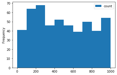
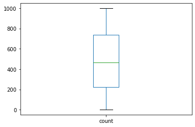
data = pd.DataFrame({'count':np.random.randint(0,1000,500)})
data.dtypes
data.plot(y='count', kind='hist')
data.plot(y='count',kind='box')
Gotchas
Always uses loc() and iloc() to do indexing/slicing to avoid confusion
Situation 1: integers as row labels
#example 1: A Series with integers as index labels.
data = pd.Series(np.random.random(5),index=[2,3,4,8,6])
data
#What will happen? we are selecting the first item or the item with a label=0?
data[0]
data.loc[2]
data.iloc[0]
Situation 2: Dataframe
#example 2: dataframe
data = pd.DataFrame(np.random.random((3,4)),columns=['a','b','c','d'], index=['a','b','c'])
data
data['a'] #returns a column
data[0]# returns what?? the first column or the first row?
data[0:1]#returns what? the first column or the first row?
Label-based slicing is inclusive
The end bound of the slice in .loc() is included, which is different from the default slicing behavior of Python.
data = pd.Series(np.random.randint(0,100,10),index=range(0,10))
data
#use iloc
data.iloc[:2]
data.loc[:2] # the end point of this slice is included.
Copy Vs. View
- All operations return a copy.
- If inplace=True is set in the caller function, the operation modify the data in place; only few operations support this setting.
- iloc[], .loc[] always modify data in place.
- Never do chained indexing when modifying data. The modifying is not guaranteed to work.
#example of chained indexing
data = pd.DataFrame({'name':['p1','p2','p3','p4','p5'],
    'state':['TX',"RI","TX","CA","MA"],
                     'income(K)':np.random.randint(20,70,5),
                    'height': [4, 5, 6.2, 5.2, 5.1]})
data
#we tried to modify the cell[0,0] to 'Mike'.
data.loc[0].loc['name'] = 'mike'
data
The reason is the first part of the chained indexing returns a copy, and the second part is modifying the returned copy (an intermediate variable) rather than the original data.
Comprehensive Project
Comprehensive Projection Solution