Pandas¶

Introduction to Pandas¶

First things first, Pandas is a package, which is the most important tool for data manipulation and analysis (Python Developers Survey 2020 Results)

The name of Pandas is derived from 'Panel Data'.

Glossary
panel data: In statistics and econometrics, panel data or longitudinal data, are multi-dimensional data involving measurements over time. 1

What is numpy and pandas¶

In terms of release time, Numpy preceded Pandas. Numpy is an open-source Python library used for scientific computing and provides high-performance operations on arrays and matrices (ndarray object). ndarrays are stored and processed more efficiently than Python's default list objects through vectorized operations.
Pandas library is built on Numpy Package, as a higher-level wrapper for the convenience of data science users. Instead Pandas abstracts away those mathematical terms (e.g., vectors, matrices) and turns them into some familiar concepts such as columns, spreadsheet. This way everybody is HAPPY!

One step further: why numpy(ndarray) is faster?¶

Requires all the elements in a ndarray object to have the same data type, either integer or floating point numbers, but not a mix of the two. This saves tremendous time inspecting if an operation is workable with specific elements.

a_list = [2,3,4,'t']
#now we want to apply x+10 to all elements of this list
result = [x+10 for x in a_list]
result

---------------------------------------------------------------------------
TypeError                                 Traceback (most recent call last)
<ipython-input-1-28563919a579> in <module>
      1 a_list = [2,3,4,'t']
      2 #now we want to apply x+10 to all elements of this list
----> 3 result = [x+10 for x in a_list]
      4 result

<ipython-input-1-28563919a579> in <listcomp>(.0)
      1 a_list = [2,3,4,'t']
      2 #now we want to apply x+10 to all elements of this list
----> 3 result = [x+10 for x in a_list]
      4 result

TypeError: can only concatenate str (not "int") to str

A TypeError was triggered. During each iteration, Python interpretor checks whether the intended operation is workable with the element. Say you have a list of 1 million elements, Python has to check the compatibility issue for 1 million times, which is a huge waste of time and computing resources. Numpy came up with a new data type to this problem that is it requires every single element in the list has to be of the same data type. This saves tons of computing time and resources. In addition, it opens the door for vectorized operations which allows more data to be processed at once.

Once Numpy knows an array's elements are homogeneous in data type, the next step Numpy does is to delegate the array to numpy's optimized C code, which is blazingly fast.

Python packages built on Numpy¶

Not only is Pandas is built on Numpy, many scientific computing packages are developed on the top of Numpy 2.

Learning Pandas¶

Numpy is only concerned with high-performance numeric computation (e.g., Matrix transpose, matrix multiplication, and so on), however, pandas is designed more for data scientists who care about data manipulation, missing data, queries, splitting and so on. For instance, some of you might be familiar with SQL statements which can be used in Pandas directly.
Also, as mentioned earlier, Pandas acts as a higher-level wrapper of Numpy cores, which intends to make the learning a lot easier.

Import pandas and numpy modules¶

import pandas as pd
import numpy as np #Some of the demos below will use functions from numpy.

pd.__version__

'1.1.3'

Pandas's Data Structures¶

Pandas has two main data structures.

Series: is a one-dimensional labeled array that is able to hold any data types (integers, strings, floating point numbers). Think of a series as a column in your spreadsheet. Did you ever pay attention to the leftmost side of a spreasheet indicating the line number/index? Series object has the same design, which in Pandas is called index. The index can be a list of integers, letters or literally anything. The values of index are called labels.

Dataframe: is a two-dimensional data structure, quite similar to a tabular spreadsheet with rows and columns. In addition to the row labels shown on the leftmost that is used to indentify rows, a dataframe object also has column labels that are used to index columns.

Essential Functions¶

Reading/Writing Data¶

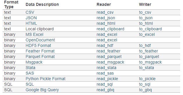
Pandas can handle virtually any data file format. Below is a table containing supported data formats and their reader & writer functions.

data formats supported

Import Parameters¶

read_csv

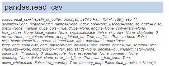
It has more than 50 parameters!? Here are some important parameters you need to pay attention to.

filepath_or_buffer: Any valid string path is acceptable. The string could be a URL. for example: Windows: "D:/data/xx.csv" OS: "usr/you/document/xxx.csv"
Tip: for Mac users, if you do not know the path of a file, you could simply drag the target file into a terminal. The prompt tells you the path of that file.
sep: Separator/delimiter to use to parse the file. Defaults to ','. If your data is TSV (tab-separated values) file, pass '\t' to this parameter.
header: the row number to use as column names. Defaults to 'infer'. If your data has no columns present in the file, set this parameter to None and then pass a list of names to the name parameter.
names: used when your data has no columns.
usecols: return a subset of the columns. Instead of reading the whole dataset, this parameter tells pandas to read the columns of your interest. It is particularly useful when you are dealing with a massive dataset.
encoding: defaults to 'utf-8'. check here to get a list of all supported encodings.

Example¶

Read a web csv file via a URL address https://raw.githubusercontent.com/s4-web/pythontraining/main/data.csv

import pandas as pd
data = pd.read_csv("https://raw.githubusercontent.com/s4-web/pythontraining/main/data.csv")

data.head()

Exploring Data¶

The first thing to do after your data is loaded into Notebook, is to get to know the basic information (e.g., the dimension, size, shape, data types of all the columns) of your data and what your data looks like roughly. All the basic information can be retrieved from DataFrame object's attributes.

Hint: What are attributes of an object? Attributes are the info/properties pre-calculated when you instantiate an object.

Getting the basic info of the data through attributes¶

shape: return a tuple representing the dimensionality of the Dataframe
ndim: return an integer representing the number of dimensions
dtypes: return a Series including the data type of each column of the DataFrame.
index: Return the index labels of the Dataframe
columns: return a list of column names

data.shape # 4 rows * 4 columns

(4, 4)

data.ndim # the dimenion of your data. If you are working with HDF5 file, you might have more than 2 dimensions.

2

data.dtypes

Name     object
Grade    object
Score     int64
ID       object
dtype: object

#Object is a data type defined by Pandas.

data.index

RangeIndex(start=0, stop=4, step=1)

data.columns

Index(['Name', 'Grade', 'Score', 'ID'], dtype='object')

Viewing the data¶

head(n): return the first n rows. It is a quick solution to get a good sense of data and also to test if your data is loaded as you expect. The parameter n defaults to 5.
tail(n): return the last n rows. The parameter n defaults to 5.
describe(percentile = None, include=None, exclude=None): Generate descriptive statistics of the included columns that summarize the central tendency, dispersion, shape, ignoring NaN values. By default, this summarization only applies to numeric columns.
mean(), sum(),min(), max(), idxmin(), idxmax(): get the mean, sum, minimum, maximum, the index of the minimum value, the index of maximum value of all columns

data.head(2)

data.tail(1)

data.describe()

data.mean()

Score    92.75
dtype: float64

data.sum(numeric_only=True)

Score    371
dtype: int64

data.max()

col1    9
col2    9
col3    6
dtype: int32

data.idxmax()

col1    row4
col2    row2
col3    row3
dtype: object

Indexing: Selecting, Slicing and Modifying Data¶

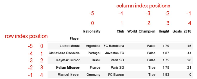
Pandas uses two indexing systems at the same time. One is the position-based indexing (starting from 0)and the other is the label-based indexing. When dealing with Series or DataFrame objects, you can use either positions (like what you do with Python on indexing a list) or labels for selecting, slicing and modifying values.

Position-based Indexing System¶

position-based indexing system

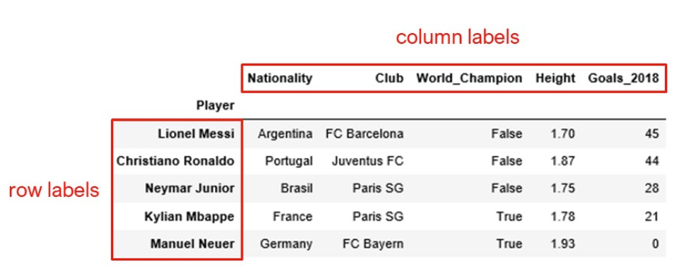
Label-based indexing System¶

label-based indexing system

Two methods for indexing¶

.iloc[]: position-based method for indexing. Allowed inputs are:
1. An integer, e.g. 5.
2. A list or array of integers, e.g. [4, 3, 0].
3. A slice object with ints, e.g. 1:7. Note the end point of the slice is not included.
4. A boolean array.
5. A callable function with one argument (the calling Series or DataFrame) and that returns valid output for indexing (one of the above). This is useful in method chains, when you don’t have a reference to the calling object, but would like to base your selection on some value.
.loc[]: label-based method for indexing. Allowed inputs are:
1. A single label, e.g. 5 or 'a', (note that 5 is interpreted as a label of the index).
2. A list or array of labels, e.g. ['a', 'b', 'c'].
3. A slice object with labels, e.g. 'a':'f'. Warning: Contrary to a python slice, For the slice in Pandas, both the start and the end slice points are included.
4. A boolean array of the same length as the axis being sliced, e.g. [True, False, True].
5. A callable function with one argument (the calling Series or DataFrame) and that returns valid output for indexing (one of the above)

df = pd.read_csv("https://raw.githubusercontent.com/s4-web/pythontraining/main/data.csv")
df.index = df.ID
df

A. passing in a single value

df.iloc[0] # returns the row-0 on the position indexing.

Name     Kevin
Grade        A
Score       99
ID        U001
Name: U001, dtype: object

df.loc['U001'] # return the row-U001 on the label indexing

Name     Kevin
Grade        A
Score       99
ID        U001
Name: U001, dtype: object

df.iloc[0, 0] #refers to the cell at position (0,0)

'Kevin'

df.loc['U001', 'Name']

'Kevin'

B. passing in a list of values

df.iloc[[0, 3]] # we want to select the row-0 and row-3 using the position indexing system

df.loc[['U001', 'U004']]

df.loc[['U001', 'U004'], ["Name", "Grade"]]

C. using a slice

df.iloc[:, 0] # return the first column,

ID
U001    Kevin
U002     John
U003     Matt
U004      Dan
Name: Name, dtype: object

df.iloc[0, :] #return the first row

Name     Kevin
Grade        A
Score       99
ID        U001
Name: U001, dtype: object

What is a boolean array? (Aka Boolean Mask array)¶

A boolean array is an array filled with True or False values. It is primarily used as a mask indicating whether the corresponding entries is selected or not.

df

x = df.Score > 85
x

ID
U001     True
U002    False
U003     True
U004     True
Name: Score, dtype: bool

df.loc[x]

df.loc[df.Score >85]

df.loc[(df.Score > 80) & (df.Name == 'Kevin')]

Syntax: In pandas, when you combine multiple conditions, you need to use & (bitwise and),| (bitwise or) or ~ (bitwise not).
Question: Why not use and to connect two criteria?

Pre-processing Data¶

Before you start to analyze your data, you might realize that you have to spend a large amount of time cleaning up data. The possible cleansing operations can be:

1. dropping irrelevant columns/rows, 
2. adding new columns/rows, 
3. fixing data missings,  dropping columns/rows in which too many missing entries are present
4. transforming certain columns E.g., add 100 to column x.

.drop(columns=, inplace=False): Drop columns by names, pass a list of names to the parameter columns. If inplace is True, the changes is operated on the original data, otherwise, a copy will be returned.
.dropna(axis='columns', how='any', thresh=None, subset=None, inplace=False) Drop columns by missings. Threshold: the minimum number of non-Nan values. subset: labels along other axis to consider.
.insert(loc, column, value): Add a new column. loc: the insertion index. Must be between 0 and len(columns)
.rename(columns={oldname: newname, }, inplace=False) Rename columns:
data.column-name.apply(func) : apply a transformation function to a certain column.

#Example
df = pd.read_csv("https://raw.githubusercontent.com/s4-web/pythontraining/main/data.csv")

df

#drop the Grade column
df.drop(columns='Grade')

df # why Grade is still in there?

df.drop(columns="Grade", inplace=True) # this time there is no return actually.

df

df = pd.read_csv("https://raw.githubusercontent.com/s4-web/pythontraining/main/data.csv")

#before we use dropna method, let's add some nan values to col_1 by using loc method
df.loc[0, 'Score'] = pd.NA #pd.NA is a data type to represent missing values.
df

df.dropna(axis='columns', how='any')

df #Rule 1: Most operations generate a copy

df.dropna(axis='columns', how='any', inplace=True) #Rule 2: if inplace parameter is present in a function, it allows you to make a inplace change.

df

#insert a new column
df.insert(value=np.random.random(4), column='col_new',loc=0)
df

#rename col_new to col_new2

df.rename(columns={'col_new':'random'},inplace=True)

df

df.sum(axis = 0)

random             2.58751
Name      KevinJohnMattDan
Grade                 ABAA
ID        U001U002U003U004
dtype: object

## Apply a function to each column to do transfromations.
#Tip: you can use a attribute-style to reference a column. E.g., data.A 
#e.g., add [1,2,3,4] to col_new2
df['random'].apply(lambda x: x+10)

0    10.454972
1    10.320459
2    10.935398
3    10.876680
Name: random, dtype: float64

df

# wait!!!! what is that? How come I get a Series object? I was expecting to get a updated dataframe. 
# Remember Rule 1? Every operation generates a copy. 
df['result']= df['random'].apply(lambda x: x+10) #rewrite the column col_new2
df

help(df.apply)

Help on method apply in module pandas.core.frame:

apply(func, axis=0, raw=False, result_type=None, args=(), **kwds) method of pandas.core.frame.DataFrame instance
    Apply a function along an axis of the DataFrame.
    
    Objects passed to the function are Series objects whose index is
    either the DataFrame's index (``axis=0``) or the DataFrame's columns
    (``axis=1``). By default (``result_type=None``), the final return type
    is inferred from the return type of the applied function. Otherwise,
    it depends on the `result_type` argument.
    
    Parameters
    ----------
    func : function
        Function to apply to each column or row.
    axis : {0 or 'index', 1 or 'columns'}, default 0
        Axis along which the function is applied:
    
        * 0 or 'index': apply function to each column.
        * 1 or 'columns': apply function to each row.
    
    raw : bool, default False
        Determines if row or column is passed as a Series or ndarray object:
    
        * ``False`` : passes each row or column as a Series to the
          function.
        * ``True`` : the passed function will receive ndarray objects
          instead.
          If you are just applying a NumPy reduction function this will
          achieve much better performance.
    
    result_type : {'expand', 'reduce', 'broadcast', None}, default None
        These only act when ``axis=1`` (columns):
    
        * 'expand' : list-like results will be turned into columns.
        * 'reduce' : returns a Series if possible rather than expanding
          list-like results. This is the opposite of 'expand'.
        * 'broadcast' : results will be broadcast to the original shape
          of the DataFrame, the original index and columns will be
          retained.
    
        The default behaviour (None) depends on the return value of the
        applied function: list-like results will be returned as a Series
        of those. However if the apply function returns a Series these
        are expanded to columns.
    
        .. versionadded:: 0.23.0
    
    args : tuple
        Positional arguments to pass to `func` in addition to the
        array/series.
    **kwds
        Additional keyword arguments to pass as keywords arguments to
        `func`.
    
    Returns
    -------
    Series or DataFrame
        Result of applying ``func`` along the given axis of the
        DataFrame.
    
    See Also
    --------
    DataFrame.applymap: For elementwise operations.
    DataFrame.aggregate: Only perform aggregating type operations.
    DataFrame.transform: Only perform transforming type operations.
    
    Examples
    --------
    >>> df = pd.DataFrame([[4, 9]] * 3, columns=['A', 'B'])
    >>> df
       A  B
    0  4  9
    1  4  9
    2  4  9
    
    Using a numpy universal function (in this case the same as
    ``np.sqrt(df)``):
    
    >>> df.apply(np.sqrt)
         A    B
    0  2.0  3.0
    1  2.0  3.0
    2  2.0  3.0
    
    Using a reducing function on either axis
    
    >>> df.apply(np.sum, axis=0)
    A    12
    B    27
    dtype: int64
    
    >>> df.apply(np.sum, axis=1)
    0    13
    1    13
    2    13
    dtype: int64
    
    Returning a list-like will result in a Series
    
    >>> df.apply(lambda x: [1, 2], axis=1)
    0    [1, 2]
    1    [1, 2]
    2    [1, 2]
    dtype: object
    
    Passing ``result_type='expand'`` will expand list-like results
    to columns of a Dataframe
    
    >>> df.apply(lambda x: [1, 2], axis=1, result_type='expand')
       0  1
    0  1  2
    1  1  2
    2  1  2
    
    Returning a Series inside the function is similar to passing
    ``result_type='expand'``. The resulting column names
    will be the Series index.
    
    >>> df.apply(lambda x: pd.Series([1, 2], index=['foo', 'bar']), axis=1)
       foo  bar
    0    1    2
    1    1    2
    2    1    2
    
    Passing ``result_type='broadcast'`` will ensure the same shape
    result, whether list-like or scalar is returned by the function,
    and broadcast it along the axis. The resulting column names will
    be the originals.
    
    >>> df.apply(lambda x: [1, 2], axis=1, result_type='broadcast')
       A  B
    0  1  2
    1  1  2
    2  1  2

##waht if I want to update the random column with the calcualted results
df['random'] = df['random'].apply(lambda x: x+10)

df

.drop(index=, inplace=False): Drop rows by labels, pass a list of names to the parameter index. If inplace is True, the changes is operated on the original data, otherwise, a modified copy is returned.
.dropna(axis='index', how='any', thresh=None, subset=None, inplace=False) Drop rows by missings. Threshold: the number of non-Nan values. subset: labels along other axis to consider.
.append(other, ignore_index=False, verify_integrity = False): Add another DataFrame to the end of the current DF. if ignore_index=True, the index of the output is reset. If verify_integration is set to True, Pandas raises ValueError on creating index with duplicates.
.rename(index={oldname: newname, }, inplace=False) Rename row labels:
.apply(func, axis=1, ) : apply a transformation function to each row. for instance, get the sum of each row.

data = pd.read_csv("https://raw.githubusercontent.com/s4-web/pythontraining/main/data.csv")

data

#drop the first two rows

data.drop(index=[0,1])

data

#add some missing values to the row_2
data.loc[0,'Grade']=pd.NA
data

#drop rows in which the the number of Non-nan is less than the threshold
data.dropna(axis=0, thresh=4) # if a row has less than 4 non-empty values, it gets deleted.

data.rename(index={1:'row_renamed'})

#try append function

df1 = pd.read_csv("https://raw.githubusercontent.com/s4-web/pythontraining/main/data.csv")
df2 = pd.read_csv("https://raw.githubusercontent.com/s4-web/pythontraining/main/data.csv")

df1.append(df2, ignore_index=False) # ignore_index=False tells Pandas to keep the data's original index labels.

df1.append(df2, ignore_index=True)

df1.append(df2, verify_integrity=True) # verify_integrity checks if those data have the duplicates on index. If so, throw out an error

---------------------------------------------------------------------------
ValueError                                Traceback (most recent call last)
<ipython-input-99-da3366c814ad> in <module>
----> 1 df1.append(df2, verify_integrity=True) # verify_integrity checks if those data have the duplicates on index. If so, throw out an error

~\anaconda3\envs\gis\lib\site-packages\pandas\core\frame.py in append(self, other, ignore_index, verify_integrity, sort)
   7741         else:
   7742             to_concat = [self, other]
-> 7743         return concat(
   7744             to_concat,
   7745             ignore_index=ignore_index,

~\anaconda3\envs\gis\lib\site-packages\pandas\core\reshape\concat.py in concat(objs, axis, join, ignore_index, keys, levels, names, verify_integrity, sort, copy)
    272     ValueError: Indexes have overlapping values: ['a']
    273     """
--> 274     op = _Concatenator(
    275         objs,
    276         axis=axis,

~\anaconda3\envs\gis\lib\site-packages\pandas\core\reshape\concat.py in __init__(self, objs, axis, join, keys, levels, names, ignore_index, verify_integrity, copy, sort)
    452         self.copy = copy
    453 
--> 454         self.new_axes = self._get_new_axes()
    455 
    456     def get_result(self):

~\anaconda3\envs\gis\lib\site-packages\pandas\core\reshape\concat.py in _get_new_axes(self)
    517     def _get_new_axes(self) -> List[Index]:
    518         ndim = self._get_result_dim()
--> 519         return [
    520             self._get_concat_axis() if i == self.bm_axis else self._get_comb_axis(i)
    521             for i in range(ndim)

~\anaconda3\envs\gis\lib\site-packages\pandas\core\reshape\concat.py in <listcomp>(.0)
    518         ndim = self._get_result_dim()
    519         return [
--> 520             self._get_concat_axis() if i == self.bm_axis else self._get_comb_axis(i)
    521             for i in range(ndim)
    522         ]

~\anaconda3\envs\gis\lib\site-packages\pandas\core\reshape\concat.py in _get_concat_axis(self)
    578             )
    579 
--> 580         self._maybe_check_integrity(concat_axis)
    581 
    582         return concat_axis

~\anaconda3\envs\gis\lib\site-packages\pandas\core\reshape\concat.py in _maybe_check_integrity(self, concat_index)
    586             if not concat_index.is_unique:
    587                 overlap = concat_index[concat_index.duplicated()].unique()
--> 588                 raise ValueError(f"Indexes have overlapping values: {overlap}")
    589 
    590 

ValueError: Indexes have overlapping values: Int64Index([0, 1, 2, 3], dtype='int64')

#apply a transformation to each values of each row
df = pd.read_csv("https://raw.githubusercontent.com/s4-web/pythontraining/main/data.csv")
df_num = df.loc[:, ["Score"]].copy()
df_num["Score2"] = [10, 20, 30, 40] # you can also use df_num.insert() method to add a new column
df_num

df_num.apply(lambda x: sum(x), axis=1) # if you feel axis is confusing, always check with help()

0    109
1    100
2    122
3    140
dtype: int64

.applymap(func): apply a function to each element of the dataframe

#get the length of each element
data = pd.DataFrame(np.random.randint(0,100, (4,3)), 
                    columns=['col_'+str(x) for x in range(3)], 
                   index=['row_'+str(x) for x in range(4)])
data

data.applymap(lambda x: x*2)

data

Missing value¶

.isull(): element-wise operation, returns a boolean Series. Detect if a value is np.nan. Tip: np.nan is a data type notation to representing nullnuess in Numpy.
.notnull(): element-wise operation. The opposite of isnull()
.fillna(value=None, method=None, axis=None,inplace=False) Fill Nan values using specified value(s) or method

Use this link to get another dataset which has missing values https://raw.githubusercontent.com/s4-web/pythontraining/main/datanull.csv

Count how many missings are present in each column¶

data = pd.read_csv("https://raw.githubusercontent.com/s4-web/pythontraining/main/datanull.csv")
data

data.isnull()

data.notnull()

#Count how many missings are present in each column
data.isnull().sum()

Name     0
Grade    1
Score    1
ID       0
dtype: int64

#Count the number of missing in each row
data.notnull().sum()

Name     8
Grade    7
Score    7
ID       8
dtype: int64

fill missings with 0s¶

data = pd.read_csv("https://raw.githubusercontent.com/s4-web/pythontraining/main/datanull.csv")
data

data.fillna(value=0)

Question: I want to replace missings in different columns differently. Replace all the missing Grade as 'B'; replace all the missing scores as 50.

data.fillna({"Grade": 'B', "Score": 50})

Fill missing with backward-fill method¶

data

data.fillna(axis=0, method='bfill') # bfill method uses the next valid value to fill the holes

Merging/Joining Data¶

.merge(right, how='inner', on=None, left_on=None, right_on=None, left_index=False, right_index=False, ): merge two Dataframe objects on a specified column/index.
.join(other, on=None,lsuffix='', rsuffix=''): Similar to the merge function, but join method can take as many dataframes as possible. The limit is it only look at the aligned index to do concatenation.
Merge Vs Join Vs. Append:
1. Merge gives you more customization power than join. You could tell this from the number of parameters. Merge method has more parameters than join function.
2. Join requires the common colummns having the same name(s). However, Merge does not have this limit.
3. The biggest advantage of using join is that you could join as many dataframes as possible.
4. Append only patch the new data to the bottom of the old data.

df1 = pd.read_csv("https://raw.githubusercontent.com/s4-web/pythontraining/main/data.csv")
df2 = pd.read_csv("https://raw.githubusercontent.com/s4-web/pythontraining/main/datanull.csv")

df1

df2

"Join" two dataframes using index¶

df1.join(df2, lsuffix="_2018",rsuffix="_2019")

"Merge" two dataframes using index¶

#merge two dfs on the index, same as the join 
df1.merge(df2, left_index=True, right_index=True, suffixes=('_2018', "_2019"))

Merge two dataframes on a common column¶

#merge two dfs on a specified common column,
df1.merge(df2, left_on="ID", right_on="ID", suffixes=('_2018', "_2019"))

Iteration of DataFrame¶

Iterate over rows:
1. iterrows(): return a pair(index, Series)
2. itertuples(): return a named tuple object: Pandas(Index=0, col_1=2, ...) (Recommended as this method preserves the data types of values. Also this method runs faster than iterrows())
Iterate over columns:
1. iteritems(): return a pair (column name, Series) paris

data = pd.read_csv("https://raw.githubusercontent.com/s4-web/pythontraining/main/data.csv")

data

Iteration over rows¶

##Example: iterate over rows
for row in data.itertuples():
    print(row.Index, row.Score) # Note that Index is capitalcase.

0 99
1 80
2 92
3 100

#Example iterate over rows using iterrows
for index, row in data.iterrows():
    print(row.Name)

Kevin
John
Matt
Dan

Iteration over columns¶

#example iterate over columns
for index, col in data.iteritems():
    print(col) #col is a series object

0    Kevin
1     John
2     Matt
3      Dan
Name: Name, dtype: object
0    A
1    B
2    A
3    A
Name: Grade, dtype: object
0     99
1     80
2     92
3    100
Name: Score, dtype: int64
0    U001
1    U002
2    U003
3    U004
Name: ID, dtype: object

GroupBy Operations¶

.groupby(by=None). The parameter by is used to dtermine how to make groups.
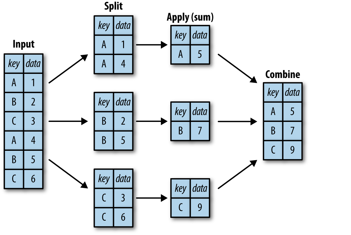
A groupby operation is a combination of splitting the object into groups, applying a function to each group, and combining the results.

The splitting step breaks up the dataframe into groups depending on the values of the specified key.
The applying step does some computing operations (e.g., transformation, aggregation(sum, std),) within each group.
The combining step merges the results of all the groups into an output dataframe.

#Example
data = pd.DataFrame({'name':['p1','p2','p3','p4','p5'],
    'state':['TX',"RI","TX","CA","MA"],
                     'income(K)':np.random.randint(20,70,5), 
                    'height': [4, 5, 6.2, 5.2, 5.1]})
data

#get the mean income and mean height of each state
data.groupby('state').mean() # Question: where is name? mean operation is not compatible with a string column.

data.groupby('state').sum()

#what if we want to apply differnt methods to differnt columns

data.groupby('state').aggregate({'income(K)':max, 'height':min })

Visualization¶

DataFrame.plot(x=None, y=None, kind='line'). The 3 most important parameters:

x : label or position, default None
y : label, position or list of label, positions, default None
kind : str
1. ‘line’ : line plot (default)
2. ‘bar’ : vertical bar plot
3. ‘barh’ : horizontal bar plot
4. ‘hist’ : histogram
5. ‘box’ : boxplot
6. ‘kde’ : Kernel Density Estimation plot
7. ‘density’ : same as ‘kde’
8. ‘area’ : area plot
9. ‘pie’ : pie plot
10. ‘scatter’ : scatter plot
11. ‘hexbin’ : hexbin plot

The plotting power of Pandas is limited compared to other Python visualization packages, e.g., Matplotlib, seaborn. Oftentimes, we only use pandas.plot function to explore data.
further reading: Overview of Python Visualization Tools

data = pd.DataFrame({'count':np.random.randint(0,1000,500)})
data.dtypes

count    int32
dtype: object

data.plot(y='count', kind='hist')

<matplotlib.axes._subplots.AxesSubplot at 0x1c08e9b3080>

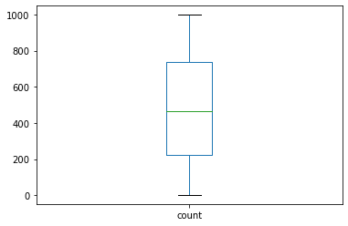
data.plot(y='count',kind='box')

<matplotlib.axes._subplots.AxesSubplot at 0x1c08e75e208>

Gotchas¶

Always uses loc() and iloc() to do indexing/slicing to avoid confusion¶

Situation 1: integers as row labels¶

#example 1: A Series with integers as index labels. 
data = pd.Series(np.random.random(5),index=[2,3,4,8,6])
data

2    0.187177
3    0.678741
4    0.737007
8    0.435342
6    0.824263
dtype: float64

#What will happen? we are selecting the first item or the item with a label=0? 
data[0]

---------------------------------------------------------------------------
KeyError                                  Traceback (most recent call last)
~\anaconda3\envs\gis\lib\site-packages\pandas\core\indexes\base.py in get_loc(self, key, method, tolerance)
   2894             try:
-> 2895                 return self._engine.get_loc(casted_key)
   2896             except KeyError as err:

pandas\_libs\index.pyx in pandas._libs.index.IndexEngine.get_loc()

pandas\_libs\index.pyx in pandas._libs.index.IndexEngine.get_loc()

pandas\_libs\hashtable_class_helper.pxi in pandas._libs.hashtable.Int64HashTable.get_item()

pandas\_libs\hashtable_class_helper.pxi in pandas._libs.hashtable.Int64HashTable.get_item()

KeyError: 0

The above exception was the direct cause of the following exception:

KeyError                                  Traceback (most recent call last)
<ipython-input-196-a9429a10ca83> in <module>
      1 #What will happen? we are selecting the first item or the item with a label=0?
----> 2 data[0]

~\anaconda3\envs\gis\lib\site-packages\pandas\core\series.py in __getitem__(self, key)
    880 
    881         elif key_is_scalar:
--> 882             return self._get_value(key)
    883 
    884         if is_hashable(key):

~\anaconda3\envs\gis\lib\site-packages\pandas\core\series.py in _get_value(self, label, takeable)
    987 
    988         # Similar to Index.get_value, but we do not fall back to positional
--> 989         loc = self.index.get_loc(label)
    990         return self.index._get_values_for_loc(self, loc, label)
    991 

~\anaconda3\envs\gis\lib\site-packages\pandas\core\indexes\base.py in get_loc(self, key, method, tolerance)
   2895                 return self._engine.get_loc(casted_key)
   2896             except KeyError as err:
-> 2897                 raise KeyError(key) from err
   2898 
   2899         if tolerance is not None:

KeyError: 0

data.loc[2]

0.01559272108993981

data.iloc[0]

0.01559272108993981

Situation 2: Dataframe¶

#example 2: dataframe
data = pd.DataFrame(np.random.random((3,4)),columns=['a','b','c','d'], index=['a','b','c'])
data

data['a'] #returns a column

a    0.503207
b    0.850066
c    0.224967
Name: a, dtype: float64

data[0]# returns what?? the first column or the first row?

---------------------------------------------------------------------------
KeyError                                  Traceback (most recent call last)
~\anaconda3\envs\gis\lib\site-packages\pandas\core\indexes\base.py in get_loc(self, key, method, tolerance)
   2894             try:
-> 2895                 return self._engine.get_loc(casted_key)
   2896             except KeyError as err:

pandas\_libs\index.pyx in pandas._libs.index.IndexEngine.get_loc()

pandas\_libs\index.pyx in pandas._libs.index.IndexEngine.get_loc()

pandas\_libs\hashtable_class_helper.pxi in pandas._libs.hashtable.PyObjectHashTable.get_item()

pandas\_libs\hashtable_class_helper.pxi in pandas._libs.hashtable.PyObjectHashTable.get_item()

KeyError: 0

The above exception was the direct cause of the following exception:

KeyError                                  Traceback (most recent call last)
<ipython-input-201-4428dd38234c> in <module>
----> 1 data[0]# returns what?? the first column or the first row?

~\anaconda3\envs\gis\lib\site-packages\pandas\core\frame.py in __getitem__(self, key)
   2900             if self.columns.nlevels > 1:
   2901                 return self._getitem_multilevel(key)
-> 2902             indexer = self.columns.get_loc(key)
   2903             if is_integer(indexer):
   2904                 indexer = [indexer]

~\anaconda3\envs\gis\lib\site-packages\pandas\core\indexes\base.py in get_loc(self, key, method, tolerance)
   2895                 return self._engine.get_loc(casted_key)
   2896             except KeyError as err:
-> 2897                 raise KeyError(key) from err
   2898 
   2899         if tolerance is not None:

KeyError: 0

data.iloc[0]

a    0.503207
b    0.230358
c    0.482812
d    0.379301
Name: a, dtype: float64

Label-based slicing is inclusive in Pandas¶

The end bound of the slice in .loc() is included, which is different from the default slicing behavior of Python.

data = pd.Series(np.random.randint(0,100,10),index=range(0,10))
data

0    19
1    64
2    88
3    37
4    75
5    40
6    15
7    75
8    60
9    76
dtype: int32

#use iloc 
data.iloc[0:2] # select the first two rows

0    19
1    64
dtype: int32

data.loc[0:2] # the end point of this slice is included.

0    19
1    64
2    88
dtype: int32

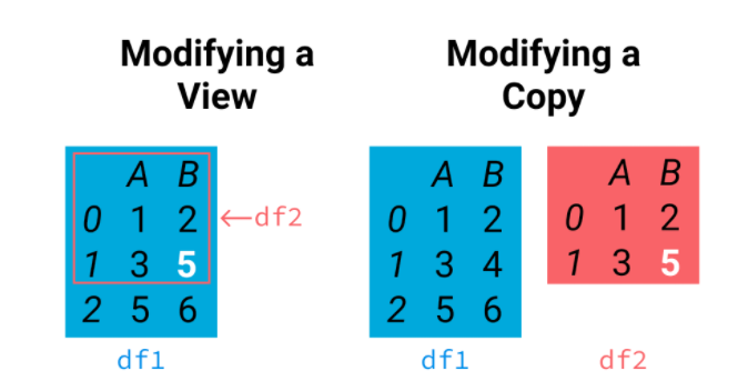
Copy Vs. View: Chained indexing¶

df = pd.read_csv("https://raw.githubusercontent.com/s4-web/pythontraining/main/data.csv")
df

Task: Change Kevin's Score to 100

#Solution1: Find the row which belongs to Kevin and then update its score
df2 = df.copy() # this creates a coopy of df
x = df2[df2.Name == "Kevin"] #Problem happens to this line. This leads to a copy, rather than a view to its orignial df2
x['Score'] = 100 
df2

<ipython-input-210-2b0e71f7147a>:4: SettingWithCopyWarning: 
A value is trying to be set on a copy of a slice from a DataFrame.
Try using .loc[row_indexer,col_indexer] = value instead

See the caveats in the documentation: https://pandas.pydata.org/pandas-docs/stable/user_guide/indexing.html#returning-a-view-versus-a-copy
  x['Score'] = 100

Where is the problem? Okay, the problem happens to the statement x = df2[df2.Name == "Kevin"]. This line returns a new copy of the selected rows. When you move to the next line where you want to update the score, it turns out you are manipulating the value of a new variable rather than the original data.
df2[df2.Name=='Kevin']['Score'] == 10 is functionally the same as the aforementioned example.

##Solution 2: squeeze all the conditions in a single loc call
df1 = df.copy() 
df1.loc[df1.Name == 'Kevin', "Score"] = 100
df1

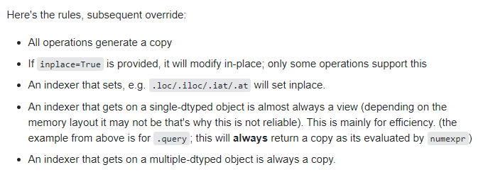
Rules to follow: Copy Vs. View (Source: Stackflow)
rules

Comprehensive Project¶

Link to the project

Comprehensive Projection Solution¶

link to the project solution

	Score
count	4.000000
mean	92.750000
std	9.215024
min	80.000000
25%	89.000000
50%	95.500000
75%	99.250000
max	100.000000

	col_0	col_1	col_2
row_0	24	118	154
row_1	12	24	106
row_2	40	20	194
row_3	180	190	156

	Name	Grade	Score	ID
0	Kevin	NaN	NaN	U001
1	John	B	90.0	U002
2	Matt	A	91.0	U003
3	Dan	A	95.0	U004
4	Kevin2	C	67.0	U005
5	John2	C	70.0	U006
6	Matt2	A	95.0	U007
7	Dan2	B	86.0	U008

	Name	Grade	Score	ID
0	Kevin	0	0.0	U001
1	John	B	90.0	U002
2	Matt	A	91.0	U003
3	Dan	A	95.0	U004
4	Kevin2	C	67.0	U005
5	John2	C	70.0	U006
6	Matt2	A	95.0	U007
7	Dan2	B	86.0	U008

	Name	Grade	Score	ID
0	Kevin	B	50.0	U001
1	John	B	90.0	U002
2	Matt	A	91.0	U003
3	Dan	A	95.0	U004
4	Kevin2	C	67.0	U005
5	John2	C	70.0	U006
6	Matt2	A	95.0	U007
7	Dan2	B	86.0	U008

	col_new	Name	Grade	ID
0	0.454972	Kevin	A	U001
1	0.320459	John	B	U002
2	0.935398	Matt	A	U003
3	0.876680	Dan	A	U004

	random	Name	Grade	ID	result
0	10.153129	Kevin	A	U001	10.153129
1	10.546070	John	B	U002	10.546070
2	10.372882	Matt	A	U003	10.372882
3	10.130736	Dan	A	U004	10.130736

	Name	Grade	Score	ID
0	Kevin	<NA>	99	U001
row_renamed	John	B	80	U002
2	Matt	A	92	U003
3	Dan	A	100	U004

	Name	Grade	Score	ID
0	False	True	True	False
1	False	False	False	False
2	False	False	False	False
3	False	False	False	False
4	False	False	False	False
5	False	False	False	False
6	False	False	False	False
7	False	False	False	False

	a	b	c	d
a	0.503207	0.230358	0.482812	0.379301
b	0.850066	0.799247	0.350966	0.343098
c	0.224967	0.498676	0.569071	0.489040